GUI: transformations

Experimental 1D signals

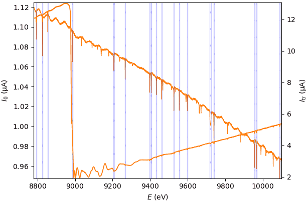
The first three transformation nodes have the same transformation widget with the only function of highlighting monochromator glitches in the present transformation node, the µd(E) node and the χ(k) node.

class parseq_XAS.XAS_widgets.CurWidget(*args: Any, **kwargs: Any)

This widget has a single tool – a panel for highlighting monochromator glitches in several transformation nodes. This tool is not a part of any transformation and only serves for visual diagnostics.

The glitch detection utilizes scipy.signal.find_peaks(). Read the tooltips of the two involved parameters.

Note

The glitch detection works only for one data object – the first one among possibly several selected.

Note

The glitch detection is implemented as static, i.e. it does not change upon changing the data selection. The change is always manual and is requested by re-checking the checkbox “mark glitches”.

Currentsµd(E)χ(k)

class parseq_XAS.XAS_widgets.HERFDWidget(*args: Any, **kwargs: Any)

This widget controls the HERFD µ calculation from a 2D data array in “scanning energy” vs “tangential detector axis” coordinates. The widget sets the parameters of two actions: level cutoff and integration within a ROI.

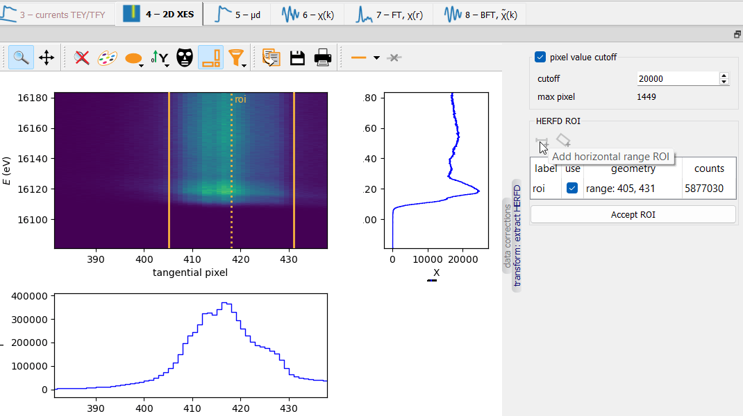
Level cutoff

Doing a cutoff can be useful if a bad pixel appears within the ROI. The side histograms can be useful in setting the level.

Caution

Examine the “max pixel” value that is calculated after applying the cutoff. It should be much less than the cutoff value, otherwise the cutoff removes a useful signal.

Integration ROI

There is a choice of two ROIs: a vertical band (horizontal range) and a slanted band. The ROI can be set by the mouse in the 2D plot and/or from the “geometry” cell in the table. The current ROI can be deleted by using the popup menu in the plot.

The calculations are done by XAS_transforms.MakeHERFD.

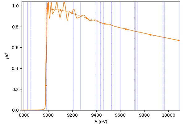
Absorption coefficient µd(E)

class parseq_XAS.XAS_widgets.MuWidget(*args: Any, **kwargs: Any)

The calculations are done by XAS_transforms.MakeChi.

Tip

The range selection widgets have an auto option and a custom selection option. The latter can be set by the mouse in the plot or by typing in the edit widget. Hover the pointer over the edit widget to discover the meaning of the min and max values: sometimes as fractions of a given range, sometimes as absolute values of a given unit etc. Similarly, a tooltip of the “auto” radio button displays the implied automatic range.

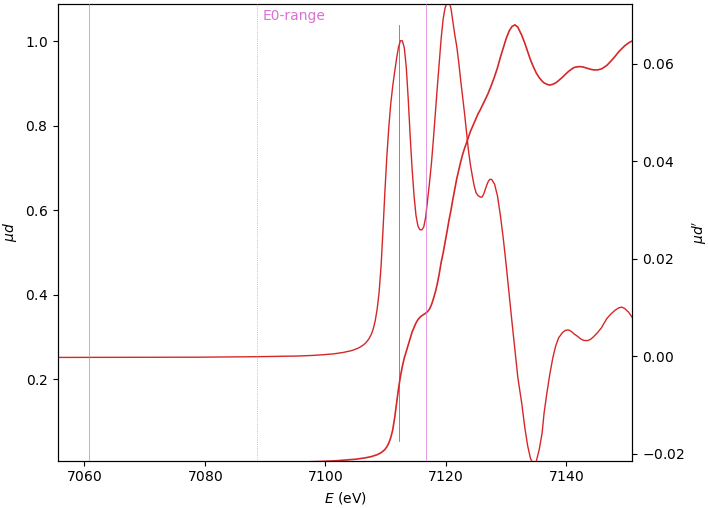
Edge position E₀

The three E₀ options give similar, still varying, results.

0: (µd)’ max	1: (spline)’ max	2: µd’ peak mean
E₀=7112.498	E₀=7112.655	E₀=7112.333

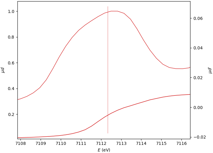
When the edge has several derivative maxima, the edge position should be placed over the first one. In this case, the E₀ search range should exclude the main derivative peak:

Energy calibration

The found E₀ position can be assigned to a tabulated value that can either be selected from the drop-down list or typed in manually. Alternatively, a shift of E₀ can be specified. The former method should be used for a reference material with a known edge position (most typically a foil), which would calculate a shift of E₀. This shift can be applied to all other spectra measured during the same beam time. The energy shift is most typically applied as a constant Bragg angle offset.

Pre-edge background

Note

When “show subtracted” is unchecked, not only the pre-edge background becomes visible, also the edge normalization is switched off and disabled.

For transmission spectra, a Victoreen polynomial \(aE^{-3}+bE^{-4}\) or a modified Victoreen polynomial \(aE^{-3}+b\) are most typical. For fluorescence spectra, the background is either constant or linear.

Pinhole correction

Tip

Find the pinhole correction widget in the “data correction” splitter widget that is initially hidden. Use a small vertical button on the left from the transformation widget.

The effect of pinholes in transmission spectra is modelled in a binary way: a fraction \(x\) of x-rays goes through pinholes without absorption and the rest of the beam is properly absorbed by the sample, which gives the transmitted intensity as: \(I_1 = xI_0 + (1-x)I_0\exp(-(µd)_{true}) = I_0\exp(-(µd)_{dist})\), from where \((µd)_{true}\) can be obtained from the distorted \(µd\): \((µd)_{true} = \ln{\frac{1-x}{\exp(-(µd)_{dist}) - x}}\).

Self-absorption correction

See the description of self-absorption correction, including its history, here.

Tip

Find the self-absorption correction widget in the “data correction” splitter widget that is initially hidden. Use a small vertical button on the left from the transformation widget.

Give a chemical formula (observe thetwo given examples). A table of scattering factors is selected for the drop-down list; the one by Chantler is recommended. The parameter “calibration energy” is where the calibration constant C is calculated. The status line below calibration energy is green if an absorption edge within the spectrum range has been found. “fluorescence energy” is at present a simple edit line, but will be a drop-down list in the future. The three angles are defined in the geometry figure.

Note

The “thin” version of the correction is much heavier in calculations.

Post-edge background and edge normalization

The post-edge background is needed for defining the edge normalization. It is constructed by a polynomial interpolation. The arguments for choosing the polynomial are the same as for the pre-edge background.

Note

The checkbox “show edge height normalized” is not an individual attribute of a data item but rather a global display property. It affects all data items.

Note

The checkbox “show edge height normalized” is disabled if the pre-edge background is shown unsubtracted.

The post-edge background can also be shown “flat” (horizontal). This can be useful for the linear combination fit and the function fit of µ(E).

Atomic-like absorption coefficient µ₀

A “µ₀ prior” curve is a step-like function, with or without a “white line”, is constructed from the absorption spectrum itself. The sharp step can be smoothened. The µ₀ prior can also be vertically displaced by applying a multiplicative factor.

Two methods are offered for the spline creation: ‘through internal k-spaced knots’ and ‘smoothing spline’. The method of a spline through knots is generally better, as it contains only low-frequency oscillations, so that χ(k) preserves all the true structural oscillations. This is not the case for the smoothing spline, where the resulting χ(k) partially loses its signal and transfers it toward µ₀, but this method is easier to use, it always “just works”.

Tip

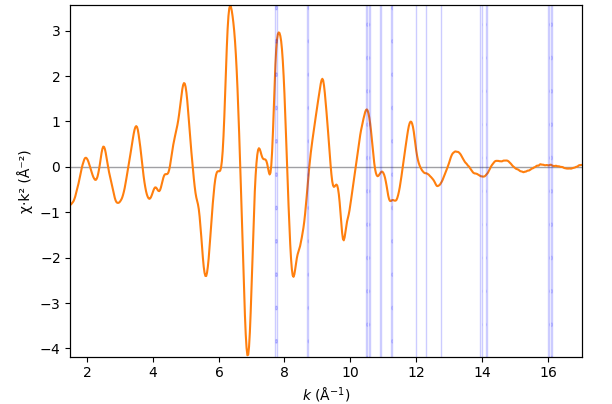
When working on µ₀ optimization, make the FT node visible by dragging it to another screen or docking it next to the µd(E) node, as on the picture below. The optimization target is to minimize the low-r portion of the FT curve, typically within the range 0 to 1 Å.

A demonstration of simultaneous observation of µd(E) and χ(r) during the optimization of µ₀.  A demonstration of simultaneous observation of µd(E) and χ(r) during the optimization of µ₀.

In the first µ₀ method (‘through internal k-spaced knots’), a given number of knots are equidistantly placed in k-space and a spline is drawn through them. The difference µ₀ – µ₀ prior is optionally weighted with a \(k^{\rm exp weight}\) factor. Additionally, a given number of the first knots can be variable in height to automatically minimize the low-r portion of the FT EXAFS. The varied knots are plotted by bigger symbols. The number of the varied knots is advised to be kept small (much smaller than the total number of knots) to make the minimization stable.

Note

The minimization sometimes becomes unstable, so that the original knots may give a better result. The reason for the failure is a very strong correlation between the knots, which makes the optimization problem poorly defined (ill-posed).

The second µ₀ method (‘smoothing spline’) depends on a smoothing parameter that is set by examining the low-r FT. By switching between the µ₀ methods, one can discover that the 1st FT peak height is always lower with the second method. This signal loss can be tolerated if it is smaller than the fitting error of the first shell coordination number.

EXAFS function χ(k)

class parseq_XAS.XAS_widgets.ChiWidget(*args: Any, **kwargs: Any)

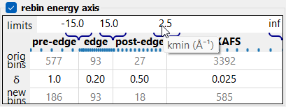
Data rebinning

 The rebin widget.

 The rebin widget.

If the energy scan was done in a continuous way with a constant slew rate, the resulted spectrum is typically strongly over sampled. This means that several experimental points fall into one dk interval of χ(k). Even more, dk intervals become larger in energy to the end of the spectrum, so more and more experimental points fall into one dk interval. These experimental points can be averaged, and this is the meaning of rebinning.

The rebinning table defines four regions by setting their limits and steps in E- or k-space.

Tip

Hover the mouse pointer to any table cell to discover the meaning of the cell value.

k range

 The k range panel.

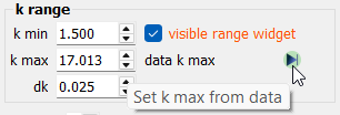
 The k range panel.

The desired k range can be set either from the spin box widgets or from the range widget in the plot.

Note

The default k max value is not set at the spectrum end. Please check the “data k max” value and use the button to maximize the range.

Denoising

Denoising utilizes scipy.signal.butter(). The two parameters, order and lowpass frequency are the first two parameters of scipy.signal.butter(). The calculated noise level is a normalized difference between the original and the denoised χ·kᵂ, see the tooltip.

FT window

The tapered FT window functions (the last three in the list) are defined by the width of the tapered part and the minimum value reached at the ends. These two parameters can be set from the spin box widgets or from the pointer widget in the plot. The pointer can be dragged in the top left quadrant of the plot.

Note

The true maximum value of the FT window function equals 1. The displayed vertical size of it is scaled to the data vertical extent, which can hinder the auto-zooming action. In this case, first hide the window, do auto-zoom and display the window again.

Fourier-transformed EXAFS function χ(r)

class parseq_XAS.XAS_widgets.FTWidget(*args: Any, **kwargs: Any)

The resulting FT is cut at a selected r max value, mainly for the plotting purpose.

The zeroth FT frequency (here, the uncorrected distance r) can be removed by nulling the first integral of χ(k); this choice is controlled by the checkbox “force FT(0)=0”.

BFT window

The BFT window function can be defined by the spin box widgets or from the range widget in the plot.

Note

The true maximum value of the FT window function equals 1. The displayed vertical size of it is scaled to the data vertical extent, which can hinder the auto-zooming action. In this case, first hide the window, do auto-zoom and display the window again.

GUI: fits

Linear Combination Fit of µ(E)

class parseq.gui.fits.LCFWidget(*args: Any, **kwargs: Any)

 A collection of reference Cu K XANES spectra and two test mixtures.

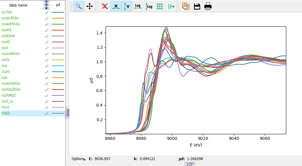
 A collection of reference Cu K XANES spectra and two test mixtures.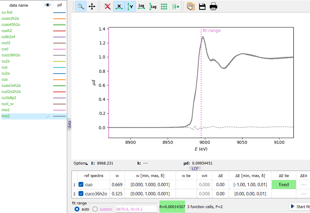 A Linear Combination Fit of a test mixture. Notice the two ways of fixing fitting parameters, here the ΔE parameter.

 A Linear Combination Fit of a test mixture. Notice the two ways of fixing fitting parameters, here the ΔE parameter.

Consider the supplied project file saved/Cu-LCF.pspj.

In this example, 16 reference Cu K XANES spectra can be used as a basis set of the linear combination fit (LCF). Two physical mixtures – mix1 and mix2 – were prepared for testing the fits.

There are two ways of adding reference spectra to the fit: from a list of spectra in the popup menu and from the data tree after the popup menu command “Add ref spectra”.

Each reference spectrum contributes with two fitting variables: weight w and energy shift ΔE. The need for ΔE, its range and interpretation remain on the user’s side. One good reason for having free ΔE’s is a possible energy variation when the spectra come from different sources.

The weights w should have their range within the interval [0, 1]. In the fit table, there is a third value – δ – that defines the view format and also sets a step for the spin box editor of the initial w value. The final values of the fitting parameters and their errors can be viewed with a higher precision by cell tooltips.

A fit variable can be fixed in three ways: by defining (a) a tie expression “fixed”, (b) a tie expression “=0.5” (or any other fixed value) and (c) the [min, max] interval with min≥max, then min is the used fixed value.

Tie expressions may also interconnect the w variables. For this purpose, they are given an integer index in brackets. Examine the tooltips of the table headers. Additionally, metavariables can be defined by the user to appear in tie expressions.

The complete fit description can be copied from one data item to other data items. The export of all fits is done by project saving. The project file is a text file of the ini-file structure; it also includes all fit settings.

Function Fit of µ(E)

class parseq.gui.fits.FunctionFitWidget(*args: Any, **kwargs: Any)

 A Function Fit example.

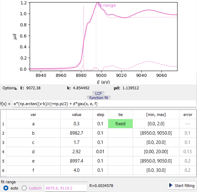 A Function Fit example.

The formula operates numpy functions as attributes of np, e.g. np.exp(x). Additionally, these functions are defined:

gau(x, m, s): normalized Gaussian function, m=center, s=sigma

lor(x, m, s): normalized Lorentzian function, m=center, s=HWHM

EXAFS Fit of χ(k) and χ(r)

class parseq.gui.fits.EXAFSFitWidget(*args: Any, **kwargs: Any)

 An EXAFS Fit example with a single coordination shell.

 An EXAFS Fit example with a single coordination shell.

Consider the supplied project file saved/Cu.pspj. In the BFT tab, press the “EXAFS fit” button under the plot, select the first data item and hide the others (press the eye header of the data tree). Press “Start fitting” to get the fit curve.

The first tab of the fit widget represents the first coordination shell (here, a single shell in the fit). The last tab contains the factor S₀² together with user metavariables.

Hover the mouse cursor over the table headers to get the description of the corresponding column.

 The correlation matrix of a single shell fit.

 The correlation matrix of a single shell fit.

The last two columns contain fitting errors: calculated (a) without pair correlations and (b) with taking account of all pair correlations. The latter should always be preferred but it may fail if the χ² function does not reach a true minimum. In such problematic cases, the table of pair correlation coefficients can be useful. It becomes visible by clicking on the error column headers. The problematic variables should be constrained or fixed.

 The FEFF-file selection dialog.

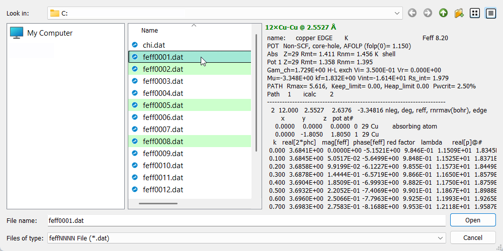 The FEFF-file selection dialog.

Each coordination shell requires a FEFF file – a file with scattering amplitudes and phases, so called feffNNNN.dat calculated by FEFF program (the ff2chi module, set its PRINT level to 3). Use the button to invoke the FEFF-file selection dialog. The dialog will search the current directory for feffNNNN.dat files and select by green color those belonging to single scattering paths. The preview panel displays the top part of the selected file, with the summary in green bold at the top. When a file is confirmed, its deg (degeneracy) and reff (r effective) parameters are set as initial values for n and r parameters of the fit shell.

Tip

It is possible to select multiple feffNNNN.dat files at once. This selection will create multiple coordination shells.

Note

Multiple-scattering paths are treated similarly to single-scattering ones. The user should apply suitable tie expressions on coordination numbers and possibly distances.

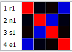
The fit operates four shell fitting parameters per shell: ‘r1’, ‘n1’, ‘s1’, ‘e1’, ‘r2’ and so on. Additionally, the global amplitude factor S₀² is represented by the variable ‘s0’. These variable names can be used in tie expressions. Examples of valid tie expressions: “fixed”, “=n1*0.5”, “>4.4-r1” (e.g. for ‘r2’ parameter, with the meaning r1+r2 > 4.4 Å).

Note

The E₀ shift parameters ‘e’ of different atomic shells should not differ much. How much is allowed depends on the calculations of the atomic potentials embedded into the calculation cluster. If the potentials were calculated self-consistently, this difference should be zero. Regardless of self-consistency, atomic shells of the same chemical element should have an equal shift.

 An example of a joint fit of two EXAFS spectra.

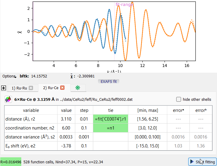 An example of a joint fit of two EXAFS spectra.

Tie expressions can refer to fits of other data items. Consider the project file saved/CeRu2.pspj where the same interatomic distance is sensed from two absorption edges. The tie expression “=fit[‘CE0074’].r1” equalizes the distance “r2” to the distance “r1” of the data item ‘CE0074’ (this is its alias). This tie expression joins the two otherwise independent fits into a bigger fitting problem. Explore its correlation matrix to discover the involved fitting parameters.